Making AI Models Explainable: Practical Use of SHAP, LIME & Other Techniques
The “black box” nature of modern AI models poses significant challenges in high-stakes applications like healthcare, finance, and criminal justice. While these models achieve impressive performance, their lack of interpretability can undermine trust, compliance, and debugging efforts. This comprehensive guide explores practical techniques for making AI models explainable, focusing on SHAP, LIME, and other powerful interpretability tools.

Why Model Explainability Matters
Model explainability has evolved from a nice-to-have feature to a critical requirement across industries. Regulatory frameworks like the EU’s AI Act and GDPR’s “right to explanation” mandate transparency in automated decision-making. Beyond compliance, explainability serves several crucial purposes:
Building Trust and Adoption: Stakeholders are more likely to trust and adopt AI systems when they can understand the reasoning behind predictions. This is particularly important in domains where human experts need to validate AI recommendations.
Debugging and Model Improvement: Explainability techniques help identify when models are making decisions for wrong reasons, relying on spurious correlations, or exhibiting unexpected biases. This insight is invaluable for model debugging and improvement.
Risk Management: Understanding model behavior helps organizations identify potential failure modes and implement appropriate safeguards. This is especially critical in high-risk applications where incorrect predictions can have serious consequences.
Domain Knowledge Validation: Explainability allows domain experts to verify whether the model’s decision-making process aligns with established domain knowledge and best practices.
Understanding the Explainability Landscape
Model explainability techniques can be categorized along several dimensions. Global vs. Local explanations represent one key distinction. Global explanations describe the overall behavior of a model across the entire dataset, while local explanations focus on individual predictions. Model-agnostic vs. Model-specific approaches offer another classification. Model-agnostic techniques work with any machine learning model, while model-specific methods are designed for particular architectures.
Post-hoc vs. Intrinsic explainability represents perhaps the most fundamental divide. Post-hoc methods attempt to explain existing models after training, while intrinsic approaches build interpretability directly into the model architecture. Each approach has its merits and appropriate use cases.
SHAP: The Unified Framework

SHapley Additive exPlanations (SHAP) has emerged as one of the most popular and theoretically grounded explainability frameworks. Based on cooperative game theory, SHAP assigns each feature an importance value for a particular prediction, representing the feature’s contribution to the difference between the current prediction and the average prediction.
Core SHAP Concepts
SHAP values satisfy several desirable properties that make them particularly appealing for practical use. Efficiency ensures that the sum of SHAP values equals the difference between the prediction and the expected value. Symmetry guarantees that features with identical contributions receive identical SHAP values. Dummy property ensures that features that don’t affect the model output receive zero SHAP values. Additivity maintains consistency when combining multiple models.
Practical SHAP Implementation
import shap
import pandas as pd
from sklearn.ensemble import RandomForestClassifier
from sklearn.model_selection import train_test_split
# Load and prepare data
data = pd.read_csv('your_dataset.csv')
X = data.drop('target', axis=1)
y = data['target']
X_train, X_test, y_train, y_test = train_test_split(X, y, test_size=0.2, random_state=42)# Train model
model = RandomForestClassifier(n_estimators=100, random_state=42)
model.fit(X_train, y_train)# Create SHAP explainer
explainer = shap.TreeExplainer(model)
shap_values = explainer.shap_values(X_test)# Generate visualizations
shap.summary_plot(shap_values, X_test)
shap.waterfall_plot(explainer.expected_value[1], shap_values[1][0], X_test.iloc[0])SHAP Explainer Types
Different SHAP explainers are optimized for specific model types. TreeExplainer works efficiently with tree-based models like Random Forest and XGBoost, providing exact SHAP values in polynomial time. LinearExplainer handles linear models and can incorporate feature correlations. DeepExplainer approximates SHAP values for deep learning models using DeepLIFT. KernelExplainer serves as the model-agnostic option, working with any model but requiring more computational resources.
SHAP Visualization Options
SHAP provides rich visualization capabilities that make explanations accessible to both technical and non-technical stakeholders. Summary plots show the most important features and their effects across all samples. Waterfall plots illustrate how individual features contribute to a specific prediction. Force plots provide interactive visualizations showing the push and pull of different features. Dependence plots reveal the relationship between feature values and their impact on predictions.
LIME: Local Surrogate Models
Local Interpretable Model-agnostic Explanations (LIME) takes a fundamentally different approach to explainability. Instead of trying to explain the entire model, LIME focuses on explaining individual predictions by learning a simple, interpretable model locally around the prediction of interest.
LIME Methodology
LIME works by perturbing the input instance and observing how the predictions change. It then fits a simple linear model to these perturbations, weighted by their proximity to the original instance. This local linear model serves as an interpretable approximation of the complex model’s behavior in the neighborhood of the instance being explained.
Practical LIME Implementation
import lime
import lime.lime_tabular
from sklearn.pipeline import Pipeline
from sklearn.preprocessing import StandardScaler
# Create and train model
pipeline = Pipeline([
('scaler', StandardScaler()),
('classifier', RandomForestClassifier(n_estimators=100, random_state=42))
])
pipeline.fit(X_train, y_train)# Create LIME explainer
explainer = lime.lime_tabular.LimeTabularExplainer(
X_train.values,
feature_names=X_train.columns,
class_names=['Class 0', 'Class 1'],
mode='classification'
)# Explain a single instance
instance_idx = 0
explanation = explainer.explain_instance(
X_test.iloc[instance_idx].values,
pipeline.predict_proba,
num_features=10
)# Display explanation
explanation.show_in_notebook(show_table=True)LIME for Different Data Types
LIME’s flexibility extends to various data types beyond tabular data. LIME for Images segments images into superpixels and determines which segments are most important for the prediction. LIME for Text perturbs text by removing words and observing the impact on predictions. LIME for Time Series can explain temporal patterns by perturbing different time segments.
LIME Considerations
While LIME offers valuable insights, practitioners should be aware of its limitations. The quality of explanations depends heavily on the choice of perturbation distribution and the locality of the linear approximation. Different runs of LIME can produce slightly different explanations due to the random sampling involved in the perturbation process. Additionally, LIME explanations are only as good as the local linear approximation assumption holds.
Other Powerful Explainability Techniques
Permutation Importance
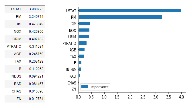
Permutation importance offers a straightforward and model-agnostic approach to feature importance. The technique measures how much the model’s performance decreases when a feature’s values are randomly shuffled, breaking the relationship between the feature and the target.
from sklearn.inspection import permutation_importance# Calculate permutation importance
perm_importance = permutation_importance(
model, X_test, y_test,
n_repeats=10,
random_state=42,
scoring='accuracy'
)# Create importance dataframe
importance_df = pd.DataFrame({
'feature': X_test.columns,
'importance': perm_importance.importances_mean,
'std': perm_importance.importances_std
}).sort_values('importance', ascending=False)Partial Dependence Plots (PDP)
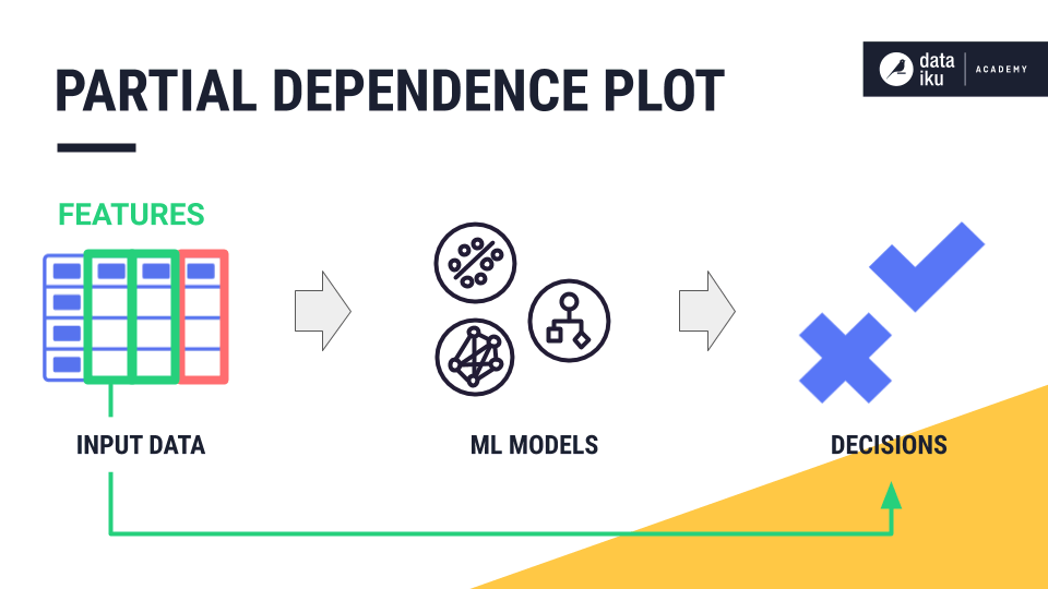
Partial dependence plots visualize the marginal effect of one or two features on the predicted outcome. They show how the model’s predictions change as specific features vary while averaging out the effects of all other features.
from sklearn.inspection import PartialDependenceDisplay# Create partial dependence plots
features = ['feature1', 'feature2', ('feature1', 'feature2')]
PartialDependenceDisplay.from_estimator(
model, X_test, features,
grid_resolution=50
)Anchors
Anchors provide rule-based explanations that identify sufficient conditions for predictions. An anchor is a set of predicates that sufficiently “anchor” the prediction locally, meaning that changes to features not in the anchor will not change the prediction.
IntegratedGradients for Deep Learning
For neural networks, Integrated Gradients computes feature attributions by integrating the gradients of the model’s output with respect to the inputs along a straight path from a baseline to the input.
Choosing the Right Technique
Selecting the appropriate explainability technique depends on several factors. Model type influences which techniques are available and most effective. Tree-based models work well with SHAP TreeExplainer, while neural networks might require Integrated Gradients or SHAP DeepExplainer.
Explanation scope determines whether you need global or local explanations. SHAP provides both, while LIME focuses on local explanations. Permutation importance and PDPs offer global insights.
Stakeholder requirements significantly influence technique selection. Technical stakeholders might appreciate detailed SHAP analyses, while business users might prefer simpler visualizations and rule-based explanations.
Computational constraints matter in production environments. Some techniques like SHAP TreeExplainer are computationally efficient, while others like LIME require more resources for perturbation-based explanations.
Implementing Explainability in Production
Production deployment of explainability requires careful consideration of performance, scalability, and integration challenges. Pre-computing explanations for batch predictions can reduce latency in real-time serving scenarios. Explanation caching can help when similar requests are common. Approximate explanations might suffice in some cases where perfect accuracy isn’t required.
Monitoring explanation quality becomes crucial in production. Sudden changes in explanation patterns might indicate data drift or model degradation, providing early warning signals for model maintenance.
Best Practices and Pitfalls
Several best practices can help maximize the value of explainability efforts. Validate explanations against domain knowledge and known relationships. If explanations contradict well-established domain knowledge, investigate potential issues with the model or data.
Use multiple techniques to gain different perspectives on model behavior. SHAP and LIME might provide complementary insights, and cross-validation between techniques can increase confidence in explanations.
Communicate uncertainty in explanations. Most explainability techniques involve approximations or sampling, and stakeholders should understand these limitations.
Avoid common pitfalls like over-interpreting local explanations as global insights or assuming that feature importance directly implies causation. Remember that explainability techniques reveal model behavior, not necessarily ground truth relationships.
The Future of AI Explainability
The field of AI explainability continues to evolve rapidly. Counterfactual explanations are gaining traction, showing what would need to change for a different prediction. Natural language explanations aim to generate human-readable descriptions of model decisions. Interactive explanations allow users to explore different scenarios and understand model behavior dynamically.
Causal inference integration represents another frontier, helping distinguish between correlation and causation in model explanations. Explanation evaluation metrics are being developed to assess the quality and reliability of different explainability techniques.
Conclusion
Making AI models explainable is no longer optional in many applications. SHAP, LIME, and other techniques provide powerful tools for understanding model behavior, but success depends on choosing the right techniques for specific use cases and stakeholders. The key lies in building explainability into the entire machine learning lifecycle, from model development through production deployment.
As AI systems become more prevalent in critical decision-making processes, the ability to explain and understand these systems becomes paramount. By mastering the techniques covered in this guide and staying current with emerging approaches, practitioners can build more trustworthy, debuggable, and compliant AI systems that serve both technical and business objectives effectively.
The investment in explainability pays dividends through improved model performance, stakeholder trust, regulatory compliance, and ultimately, more successful AI implementations that benefit both organizations and society.
Sources: datascientest.com, linkedin.com, ai.plainenglish.io, dataiku.com, technorizen.com.


No comments:
Post a Comment